


While it seems like the market chugs higher every day, it still can be buffeted by headline reading the virus spread and the pace of economic recovery. Likewise, an options value can fluctuate greatly as variables such underlying stock price and implied volatility change.
But, as an option trader one thing that never stands still is time. Learning how to harness time decay, or what is known as an options’ theta can be a powerful tool for producing consistent profits. Let’s take a look at how it works.
Time is a key component in an option’s valuation. Thankfully, it is applied equally to all options — regardless of the underlying security. But, there is one nuance that needs to be understood. In the options world time curves, accelerating as expiration approaches.
Anyone that’s ever been on a deadline can relate to that. The tool we use to define time is called theta, and it measures the rate of decay in the value of an option per unit of time.
There’s a basic math formula used in the Black-Scholes model that is a good starting point. Basically, we use the square root of time to calculate and plot time decay. The math involved in the nitty-gritty of evaluating theta can be extremely complex, so focus on this: Time decay accelerates as expiration approaches, meaning that theta is defined on a slope.
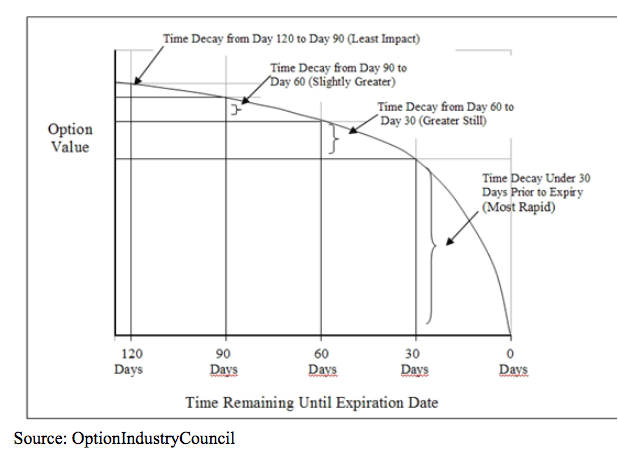

For example, if a 30-day option is valued at $1.00, then the 60-day option would be calculated as $1 times the square root of 2 (2 because there is twice as much time remaining). So, all else being equal, the value of the 60-day option is $1.41, or $1 times 1.41 (1.41 is the square root of 2). A 90-day option would be $1 times the square root of 3 (3 because there is three times as much time remaining) for an option value of $1.73. (1.71 is the square root of 3).
If you notice, the premium of the 60-day over the 90-day ($0.32) is less than that of the 60-day over the 30-day ($0.41). So again, the important takeaway is that the closer an option gets to expiration, the rate at which time value decays gets faster.
This graph makes the math easier to visualize and also shows that the rates of decay are different depending upon whether an option is in-the-money, out-of-the-money, or at-the-money.
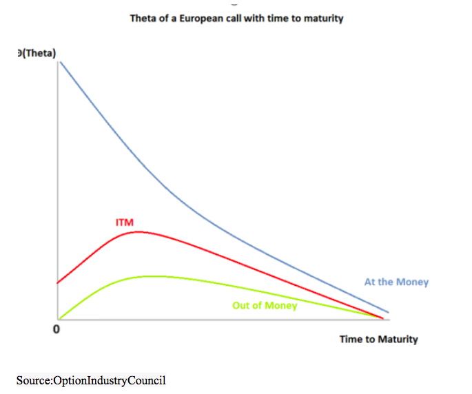

Another conclusion that can be drawn from the above charts is that, if one sells out-of-the-money options with a slightly longer-term horizon, he might plan on covering them before expiration — perhaps just past the half-way point, or so. He would do this because a large majority of the time value decay would already have taken place, and therefore, the remaining opportunity would not be as great.
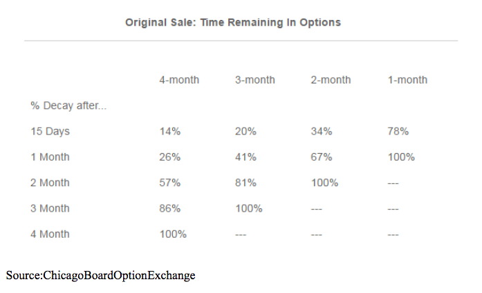
For example, suppose XYZ is trading at 100, and you sell the out-of-the-money combo, utilizing the calls with strike 120 and the puts with strike 80. The following table shows how much (unrealized) profit you would have from the naked sell combo if the stock was still at 100 one month, two months, etc.

Here are some other basic concepts you need to know about theta:
- An option’s theta can be calculated as follows: If a particular option’s theta is -10, and 0.01 of a year passes, the predicted decay in the option’s price is about $0.10 (-10 times 0.01 is 0.10).
- At-the-money options have the highest theta. Theta decreases as the strike moves further into the money or further out of the money. In-the-money options are mostly composed of intrinsic value (the difference between the strike price of the option and the market price of the underlying), while out-of-the-money options have a larger implied volatility component.
- Theta is higher when implied volatility is lower. This is because a high implied volatility suggests that the underlying stock is likely to have a significant change in price within a given time period. A high IV artificially expands the time remaining in the life of the option, helping it to retain value.
Time is always moving. In our daily lives, some days seem to pass quicker than others. So too with options.
Click here to learn more about author Steve Smith’s unique and profitable options trading approach—the Options360 service.